Intuition and math behind DeFi AMM curves
Automatic Market Makers (AMM’s) power the largest DeFi protocol in the world, Uniswap. The simple technology behind them powers billions in daily dollar volume and has created a similar amount of wealth for protocol founders.
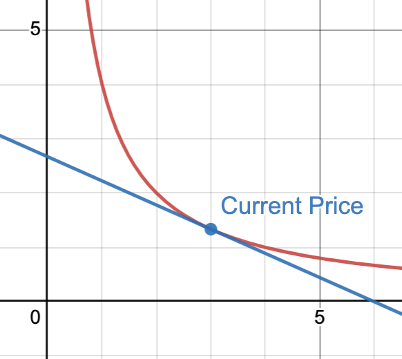
You may have seen the equation X*Y=K, or a curve like below:
But what does this chart actually represent? When the dot moves, what does that mean? How about if the curve is closer or further from 0? What does the blue line mean?
If the above chart confuses you, either a little or a lot, this post is for you. We’re going to dive into what it means, and how to interpret it. By the end of this post, you’ll have a strong intuitive understanding of the billion dollar idea behind an AMM curve.
MM vs. AMM
An AMM is an automatic market maker, but what’s a market maker? In traditional finance, a market maker (MM) is a company that is always willing to buy and sell a stock. Suppose you own a share of TSLA and want to sell it. Who’s going to buy it? Maybe you’ll get lucky and someone wants to buy TSLA at the same time you want to sell it, but that’s uncommon. Usually, you are selling to a market maker.
Suppose the fair price for TSLA shares is around $100. A market maker is willing to buy them for $99, and sell them for $101. His goal is to make pennies on the dollar by buying and selling around the spread.
The market maker provides liquidity in the market. If you want to sell $1 million shares of TSLA, you don’t have to wait around for someone who wants to buy $1 million shares of TSLA. The market maker will buy them from you, and sell them off later for a 0.1% profit. That profit is a convenience charge for being able to quickly buy and sell your shares.
In web3, an automatic market maker (AMM) provides the same function. When you do a swap on Uniswap, you never trade with counterparty. Instead, you are always buying from (or selling to) the AMM, a computer algorithm on the blockchain. The AMM buys and sells all day long, never gets tired, and never declines a trade. And unlike a traditional market maker, the AMM runs with zero human intervention.
With this background knowledge, let's dig into the mechanics of the AMM.
Simple linear AMM
To start off, let’s consider the simplest type of AMM, which is called the linear sum AMM.
Suppose the UNI price is $4, and I want to make an AMM that buys and sells at that price point all day long. No customer is ever turned down.
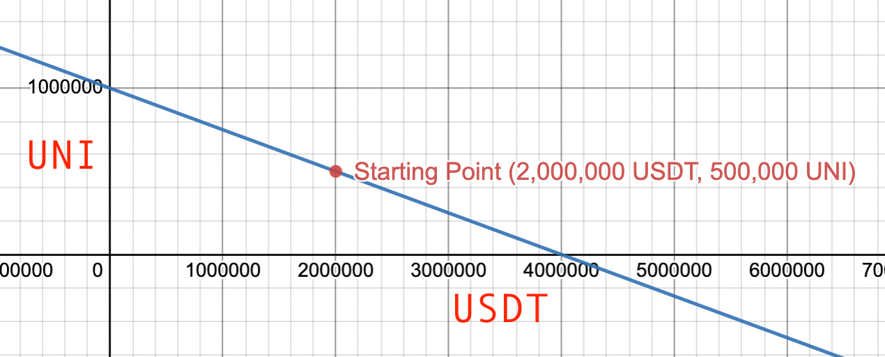
I have $4 million in capital to bootstrap this AMM, and I split it evenly between UNI and USDT for 500,000 UNI and 2,000,000 USDT. We can draw this on a chart:
The chart above shows how many tokens are in the AMM’s account. The X axis is the UNI balance, and the Y axis is the USDT balance. We start at the red dot on the chart. The further to the right we are, the more USDT the AMM’s account has. Further up means more UNI. This is the first important concept to understand an AMM: the current point is the current balance. We’ll see later how trading with the AMM moves the current point, representing changes in the AMM account balance.
For the linear sum AMM, we’re going to be naive. We write up a smart contract with the following logic:
If someone comes with $4, I’ll give them 1 UNI
If someone comes with 1 UNI, I’ll give them $4
These prices are good for any quantity of trade
This is a linear sum AMM, and it always makes trades for $4 per UNI. This behavior is represented by the equation x + 4y = 4,000,000, and shown in the chart below:
The blue line above represents the second important concept in understanding AMM’s: the slope is the exchange rate. The AMM’s current point, representing its account balance, moves along the blue line when it makes trades. When it moves to the right, it is increasing its balance of USDT while decreasing its balance of UNI. Conversely, when it moves to the left, it is increasing its balance of UNI while decreasing its balance of USDT.
How steep or flat the line is represents the current exchange rate. In the example above, the AMM will trade 1 UNI for 4 USDT, hence the slope of -¼.
The AMM contracts ensure that it never moves off the blue line. Aside from changes in liquidity, that blue line represents all the possible account balances that the AMM can have when a user trades with it.
Now that our AMM is open for business, let’s do the first trade. A seller comes along, and he wants to sell 200,000 UNI. Our AMM makes this trade at the price of 4 UNI per USDT, so the seller gets 800,000 USDT.
The green point above shows the AMM’s new position: it has 2,800,000 USDT and 300,000 UNI. We can add some more arrows to show the change on each axis:
The green arrow above shows the AMM’s gain of 200,000 UNI, and the red arrow shows the AMM’s loss of 800,000 USDT. Since the AMM did this swap at the fair market price, $4 per UNI, its account value did not change. All is well in the universe.
Let's break the linear AMM
After the first trade, our AMM is at the following point on the liquidity curve:
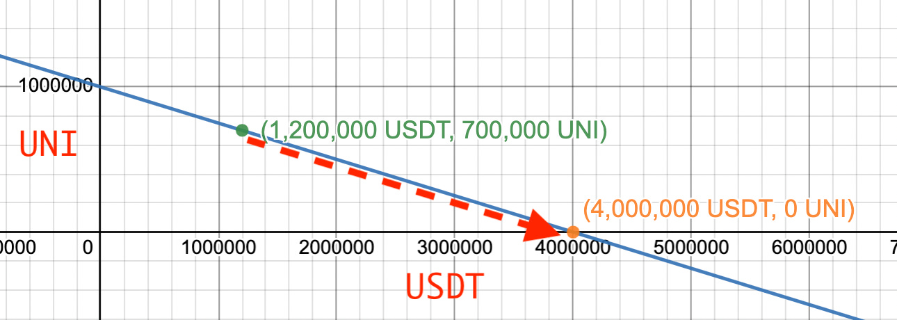
The point represents available liquidity of 1,200,000 USDT and 700,000 UNI. A buyer comes along, looking to buy 700,000 UNI. The AMM will make the trade at $4 per UNI, so the buyer deposits 2,800,000 USDT. The AMM moves to a its new point on the liquidity curve:
The AMM’s new balance is 4,000,000 USDT, and 0 UNI. The net account value is the same, but there’s a problem: the AMM is all out of UNI. If someone wants to buy UNI, they’re out of luck. The AMM has none to sell. This breaks one of the goals of the AMM which was:
The AMM never declines a trade
Until someone sells some UNI, the AMM is closed for business. Bad news.
And there’s another problem. Let’s say the value of the UNI token drops, and UNI tokens are only worth $3 now. The AMM is set to buy UNI at $4, all day long. Someone could buy a bunch of UNI token on Binance for $3, sell it to our AMM for $4, and make a nice profit. More bad news.
The linear sum AMM is simple and easy to understand, but it isn’t ready for the real world.
Enter the constant product AMM
Recall the formula powering the linear sum AMM:
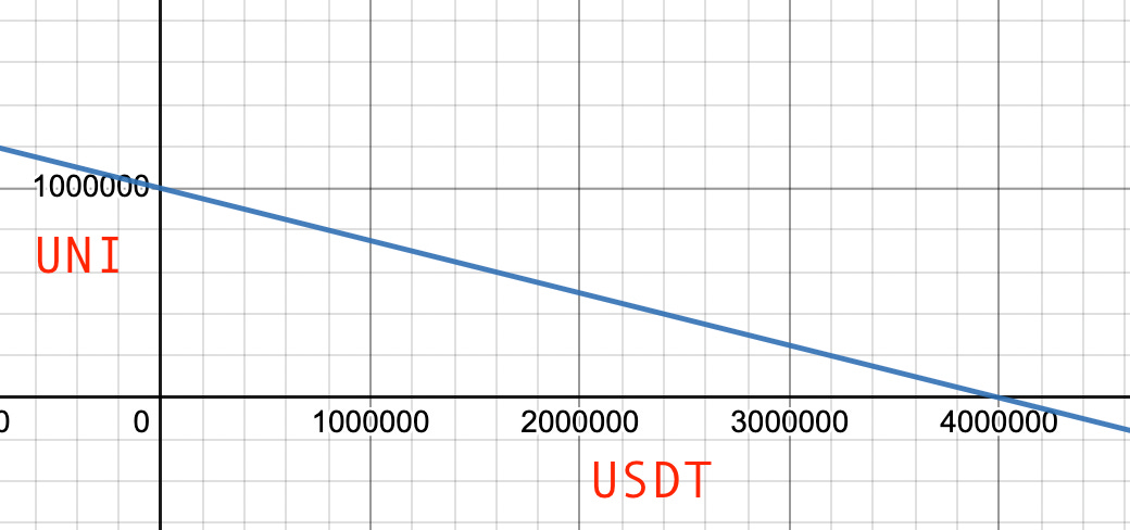
x + 4y = 4,000,000
This formula results in the following liquidity curve:
As we saw above, we hit a problem at the two axis intercepts, where the AMM is out of capital of the respective tokens:
The other problem we saw was the fixed price, which makes the AMM vulnerable to arbitrage. The slope is the price in AMM’s, and a linear function has a constant slope.
We need a more robust AMM function to solve these two problems. We’re going to add two requirements for our AMM function:
It must never touch the X or Y axis. Touching either axis means the AMM has exhausted liquidity of a token. By staying off the axes, we ensure infinite liquidity.
The price must move against the market. When the AMM sells the X axis token, its price should go up. When the AMM buys the X axis token, its price should go down. This must be reflected in the slope: buying from the AMM on the X axis (moving left) must make the slope steeper, and selling to the AMM on the X axis (moving right) must make the slope flatter.
A function that matches both these criteria is a constant product function, like x * y = k.
Let's set this up with the same capital as before of 2,000,000 USDT and 500,000 UNI:
In this chart, we start out at the same point as before, representing our initial capital.
The lines in this chart are different, however. The linear sum AMM had a single line, representing both the current price (the slope), and the range of possible account balances.
The constant product separates these two concepts into different curves. The orange line represents the possible account balances of the AMM. We will be moving along the orange line as the AMM’s account balance changes. The blue line is the slope at the current point, representing the price at that point. As the current point changes, so does the slope, and therefore the price. You may have heard the mathematical term for this line: the tangent.
Observe how this new curve meets both our requirements. The orange line can get infinitely close to either axis, but it can never touch them. That is because there is no solution for x = 0 or y = 0 to our constant product function; solving that would require division by zero.
We also meet the second requirement, which is that the price must change inversely with changes in token balance. When the balance of UNI goes down, the price of UNI must go up. When the balance of USDT goes down, the price of USDT must go up. We can observe this by seeing the change in the slope of the tangent.
Let’s revisit the example that broke the linear sum AMM by draining its UNI balance to zero. Suppose the AMM starts at 2,000,000 USDT and 500,000 UNI. A buyer comes along, looking to spend 2,000,000 USDT in exchange for UNI. In the linear sum AMM, the 4:1 exchange rate would have resulted in a movement to 4,000,000 USDT and 0 UNI.
The AMM accepts the payment of 2,000,000 USDT, just like before. However, this time, it only pays out 250,000 UNI in this trade. The price for the buyer was 8 USDT per UNI, two times what the linear sum AMM charged for the same trade.
That’s not all. 8 USDT per UNI is the average price over this one trade. At the new point on the AMM’s liquidity curve, the slope is much more flat, representing a new price of 16 USDT per UNI for the next buyer to come along.
Next concepts
This introduction explained the basic math behind AMM curves. In the next part, we’ll explore more advanced concepts, including alternate product functions, and mapping AMM liquidity to a traditional market making liquidity. Check back soon.


